In this use-case we copute IV-characteristics and analyze excitonics in a phosphorescent OLED device. The device setup, consisting of an HTL (red), an EML (host material doped with 15% (mol) emitter) and an ETL, is illustrated below. For simplicity, we did not include doped injection layers explicitly, but used effective electrodes instead. These effective electrodes have energy levels of doped injection layers and require a compensation of the modified built-in voltage. Check out our tutorial on full ab-initio stack simulation to learn how to explicitly include doped injection layers. Transport levels are given in the table below. For excitonic properties, we will apply presets.

Setup
We simulate charge carrier and exciton dynamics of this phOLED using our multi-purpose kinetic Monte-Carlo tool LightForge. The following description highlights the most relevant settings. For a general introduction to the LightForge GUI, please refer to the LightForge documentation. Further, you can find this workflow pre-defined in our virtual lab (request a free trial here). For a detailed step-by-step guide, please follow our recorded webinar, which also contains more details on analyzing simulation results.
General and IO:
- In the general-tab, set device_layout to “stack”, set_PBC to “automatic, check “connect_electrodes” and activate all particle types by checking the respective check boxes (electrons, holes and excitons)
- In the IO-tab, disable “use QP output” and “Override Settings”
We define materials, as listed above, in the materials tab. Use the “+”-button to add three more materials. If material properties are not taken from ab-initio calculations (i.e. QP output), you need to supply energy transport levels (IP, EA), energy disorder (sigma) and reorganization energies manually, using the option “PAR: eaip,sig,l” in the “input_mode_transport” dropdown menu. As illustrated below for host and emitter, we set disorder to 90 meV and lambda (reorganization energy) to 200 meV for all materials and take transport levels from the table above.
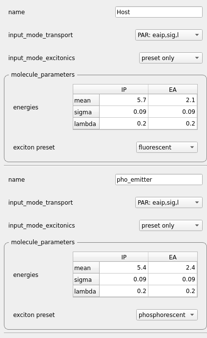
Excitonic properties are assigned to materials via presets by choosing “preset only” in the “input_mode_excitonics” dropdown menu. Available predefined presets are fluorescent, phosphorescent, doping and tadf. If required, you can add your own preset by clicking “show exciton_presets” and use the plus button to add a new preset (see e.g. the TTF-OLED use-case). For HTL, Host and ETL, set exciton preset to fluorescent. For the phosphorescent emitter, set preset to “phosphorescent”. Please refer to the webinar and the pre-defined workflow in SimStack for further details.
With the remaining tabs, proceed as follows:
- device: set morphology width to 20 nm, define all layers and adapt thicknesses according to the illustration above. Make sure to include both host and emitter in the emission layer. Set the electrode workfunctions to -5.0 eV and -2.8 eV (effective electrode, as described above), set coupling model to “parametrized” and increase electrode_wf_decay_length to 0.5.
- Topology: set “max neighbors” to 26, chose “Miller-Abrahams” as transfer integral source and leave FRET as is. Then use the plus button to add a set of pair parameters fo all material pairs (HTL-HTL, HTL-Host, HTL-Emitter, Host-Host, Host-Emitter, Host-ETL, Emitter-Emitter, Emitter-ETL, ETL-ETL). Set “maximum_ti” to 0.0003 for only the Dexter transfer integrals of all pairs and leave the rest as is.
- Physics: set rates to “automatic” and uncheck “superexchange”.
- In the Operations tab, set number of simulations to 15 to average over 15 independent runs (disorder configurations) for statistics. Set initial holes and electrons to 0, and chose fields at 0.06, 0.07, 0.08, 0.1 V/nm. Considering the modified in-built voltage of (2.8-5.0) eV, this corresponds to effective fields of 0.005, 0.015, 0.025 and 0.045 V/nm. Adapt computational parameters as follows: IV_fluctuation: 0.000001; max_iterations: 600000; max_time: 1.0e5.
- In the analysis tab, check “exciton lifecycle”, set autorun_start to 0.1 (tracking will start at 10% of the simulation time) and keep the remaining options disabled.
Now we are ready to go. Allocate up to 61 cores in the resources tab (we have 4 fields with 15 simulations each, plus one master thread) and submit the workflow to your computational resource.
Results
LightForge generates a variety of output files for analysis. In the following, we will present the output most relevant for excitonics analysis in OLED devices. For further information on outputs, please reference the LightForge documentation or send us an email. You can get results either by downloading the file “results.zip” from the runtime directory, or locating the submitted workflow in the Jobs&Workflows panel form SimStack and opening files via the SimStack filebrowser (right click on “lightforge2” in the workflow -> Browse directory).
IV and IQE, located in “results/experiments/current_characteristics” are displayed below. We find an internal quantum efficiency of almost 80% at low current density, which drops to 10% at high current density.

To investigate microscopic reasons for this roll-off, we analyze the quenching profiles, namely the files “quenching_density_average_*.png” and “exciton_decay_density_average_*_species_total.png” in the folder “results/experiments/particle_densities/”, where the *=0,1,2,3 correspond to the different fields. These profiles are compiled below for the lowest and the highest applied field.
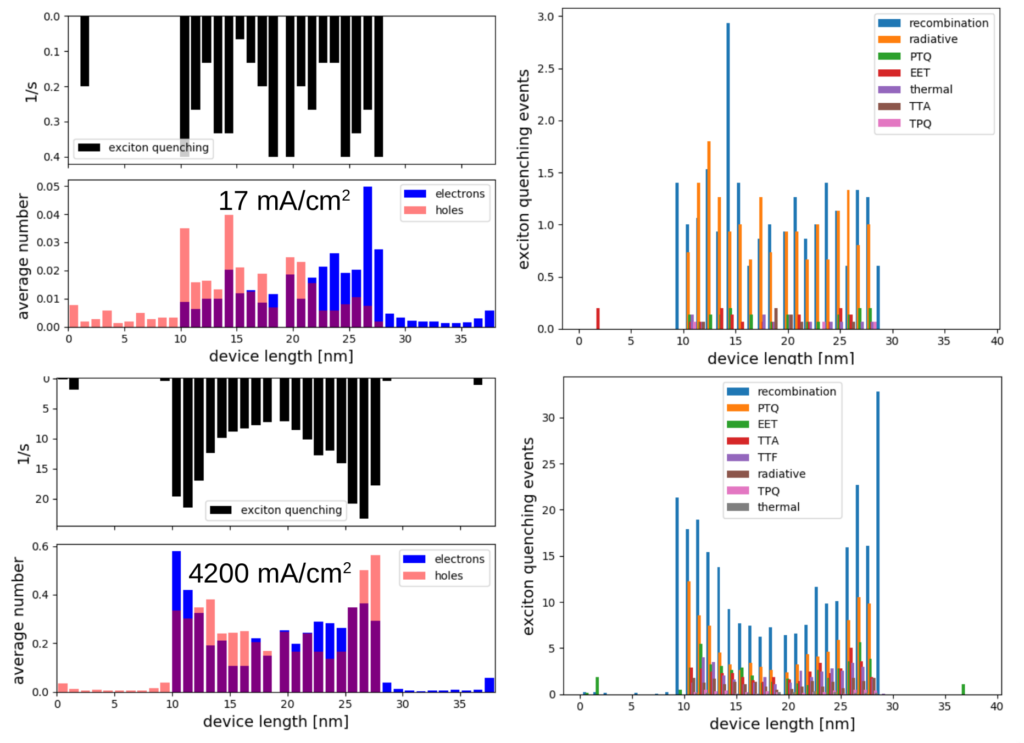
We find that the charge density in the EML at high field is approximately one order of magnitude higher than at low field. As indicated in the detailed quenching profiles on the right side, this leads to an increase in polaron-quenching, in addition to increased TTA events due to higher exciton density. Both effects result in an overall lower IQE.
For further ways to analyse your results check out our webinar or refer to the documentation page.