The aim of this application is the prediction of the charge carrier mobility for Alq3 and CBP, which is comparable with a TOF “measurement”. We need to follow a sequence of individual “virtual experiments” to compute charge carrier mobility:
- Synthesis of the molecule (Parametrizer, DihedralParametrizer)
- Thin film generation with physical vapor deposition (Deposit)
- Spectroscopic characterization and mobility measurements (QuantumPatch, lightforge)
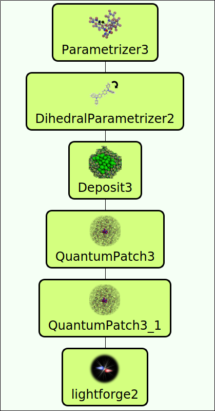
The corresponding simulation workflow is presented in Figure 1, constructed via drag&drop in our workflow platform SimStack (download available here). For this usecase, SimStack contains a predefined workflow where required settings of each individual calculation are already set. For further details of the setup of this calculation and its settings, a more detailed description of the computation of the mobility of a-NPD can be found on our documentation page.
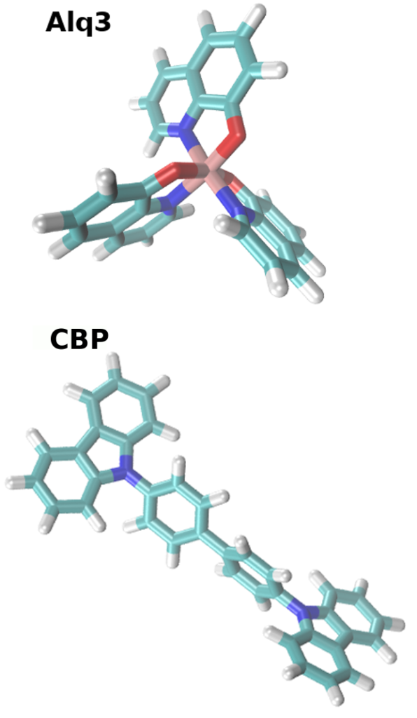
The starting point is the chemical structure of CBP and Alq3, visualized in Figure 2. We repeat the workflow depicted above for each material separately, but skip the DihedralParametrizer for Alq3 due to its rigidy. As a first step for both materias, we use the Parametrizer tool to calculate quantum chemical properties required for forcefield generation, such as the partial charges of the atoms, and optimize the molecular geometry. Different levels of quantum chemical calculations can be selected.
- As input for the Parametrizer you can use a pre-optimized 3D structure either generated with our “synthesis” equivalent tool in the mol2 format, or use the input provided in the trial version. The Parametrizer generates two relevant files: molecule.pdb and molecule.spf. molecule.pdb contains the optimized molecular configuration and molecule.spf is the force-field file for modeling the intermolecular interaction in Deposit.
Afterwards, the DihedralParametrizer characterizes the intra-molacular interaction to later sample correct molecular configurations during the deposition of the molecules in the next step:
- Load molecule.pdb and molecule.spf in the DihedralParametrizer module to generate customized energy profiles for rotation of flexible side groups of your molecule. The relevant output of the DihedralParametrizer module is a file named dihedral_forcefield.spf, which contains forcefield parameters for the intramolecular interaction, in addition to the intermolecular interaction copied from the molecule.spf of the Parametrizer output.
The next step is the formation of the morphology using the Deposit module, which mimicks physical vapor deposition by adding molecules one by one into an initially empty box. Typical thin film samples contain 1000-2000 molecules and are roughly 10-20 nm in height.
- In this example we deposit 1200 molecules into a box with dimensions set to Lx=40, Ly=40, Lz=120 (in Angstrom). These settings result in a morphology ranging from -40 A to +40 A in x and y-direction. As input for Deposit (Molecules tab), use molecule.pdb from the Parametrizer module and the dihedral_forcefield.spf from the DihedralParametrizer module, or molecule.spf of Parametrizer in case of rigid molecules.
The main results of Deposit is a sample for the spectroscopy-type calculations, performed with QuantumPatch (QP) and lightforge (lf). As indicated in the workflow-picture above, we perform two QP runs due to computational efficiency. For both runs, only the file structurePBC.cml from Deposit is required as input:
- In the first QP calculation the intermolecular couplings between 80 molecules in the center of the morphology are computed. The calculation is performed using DFT with a BP86 functional and a def2-svp basis set, as implemented in the embedded Turbomole software. To take into account the electrostatic environment of all molecules, surrounding molecules can be included with different levels of theory. In this example all molecules which are in a sphere of 15 A around the 80 molecules in the core-shell can be also treated with the same level of theory as the core shell. All molecules in a range of 25 A are calculated dynamically (their electronic structure also responds to surrounding molecules) using DFTB+ for CBP or XTB for Alq3, and all other molecules, which are more than 25 A but less than 60 A outside the core-shell are included as static point charges. Further details of the QP calculations are explained here.
- In the second QP job we compute the disorder of the orbital energies of 150 molecules using DFT with B3LYP and a def2-svp basis set, as implemented in the Turbomole software. The surrounding molecules are treated as in the first QP run.
The last step in this set of virtual experiments is the simulation of charge carrier dynamics using the lf package, resulting in the mobilities of the materials.
- Main input for the lf simulation are the files Analysis.zip from the QP runs along with the molecule.pdb of the corresponding material from the Parametrizer run. Besides many model-related settings, you can specify temperature and applied electric field in the operations-tab. Check out all required settings to compute hole mobility for the Alq3 or CBP morphology in the downloaded pre-defined examples. Further explanations of the software tool are presented here. The lf run creates a folder results, which contains among various analysis the subfolder experiments/current_characteristics where you can find mobility.png and mobilities_all_fiels.dat, presenting the final results of this study.
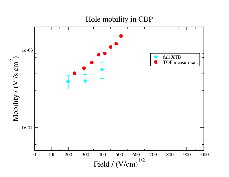
As depicted in the following figure, computed hole mobility of CBP show good agreement with the experimental measurements of Ref. 1. The employed level of theory (mix of DFT and semi-emperical methods) was a compromise between accuracy and computational efficiency. The match between the calculation and the experiment should improve further when substituting semiemperical methods for DFT.
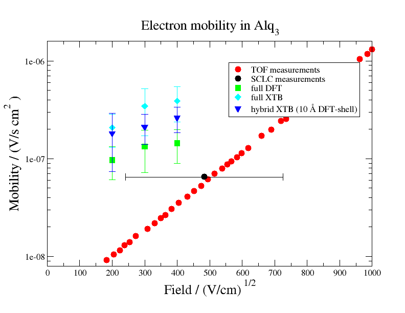
The mobility of Alq3 was calculated using the same workflow (skipping the DihedralParametrizer module) , however testing different levels of theory in the QP calculations: (i) a QP setup in which only DFT calculations are used (full DFT, green squares) (ii) a QP setup, in which only the core molecules are calculated with DFT and surrounding molecules are ccomputed with XTB (full XTB, cyan diamonds) and (iii) a mixed QP setup, in which the core molecules and molecules within 10 A of the core shell are calculated with DFT, while surrounding molecules are calculated with XTB (hybrid XTB, blue triangles).
The following figure shows these mobilities computed with LF in comparison to experimentally measured electron mobilities of Alq3 (TOF and SCLC measurement of Ref. 2, 3). The comparison shows that the simulation slightly overestimates the measured mobility. Additionally we find that mobilities from the full DFT run are closer to experimental values than mobilities from cheaper calculations, indicating that there is a dependency between accuracy and employed level of theory.
1. A. Hoping Appl. Phys. Lett. 92, 213306 (2008)
2. P. Friederich, Adv. Mater. 2017, 29, 1703505
3. H. H. Fong and S. K. So, J. Appl. Phys. 100